Reproducible Measurement of Adipose Tissue Volumes in Genetic and Dietary Rodent Obesity Models
David H. Johnson, Chris A. Flask, Paul R. Ernsberger, Wilbur Wong, and David L. Wilson
This is an author's electronic pre-print of the following publication. JMRI allows pre-prints to be shared through individual author's websites; for terms, please see this website's license. Please cite the published work as:
Johnson DH, Flask CA, Ernsberger PR, Wong WC, Wilson DL. Reproducible MRI measurement of adipose tissue volumes in genetic and dietary rodent obesity models. J Magn Reson Imaging 2008;28(4):915-927. PMID: 1188821617. DOI: 10.1002/jmri.21481.
Address for correspondence: David L. Wilson, Ph.D. dlw@case.edu.
ABSTRACT
Purpose. To develop ratio MRI [lipid/(lipid+water)] methods for assessing lipid depots and compare measurement variability to biological differences in lean controls (spontaneously hypertensive rats, SHRs), dietary obese (SHR-DO), and genetic/dietary obese (SHROBs) animals.
Materials and Methods. Images with and without CHESS water-suppression were processed using a semi-automatic method accounting for relaxometry, chemical shift, receive coil sensitivity, and partial volume.
Results. Partial volume correction improved results by 10-15%. Over six operators, volume variation was reduced to 1.9 ml from 30.6 ml for single-image-analysis with intensity inhomogeneity. For three acquisitions on the same animal, volume reproducibility was <1%. SHROBs had 6X visceral and 8X subcutaneous adipose tissue than SHRs. SHR-DOs had enlarged visceral depots (3X SHRs). SHROB had significantly more subcutaneous adipose tissue, indicating a strong genetic component to this fat depot. Liver ratios in SHR-DO and SHROB were higher than SHR, indicating elevated fat content. Among SHROBs, evidence suggested a phenotype SHROB* having elevated liver ratios and visceral adipose tissue volumes.
Conclusion. Effects of diet and genetics on obesity were significantly larger than variations due to image acquisition and analysis, indicating that these methods can be used to assess accumulation/depletion of lipid depots in animal models of obesity.
Keywords: Obesity, small animal imaging, partial volume effect, image processing, chemical shift imaging, body composition.
INTRODUCTION
Obesity has reached epidemic proportions, and it is associated with many serious medical conditions, including high blood pressure, diabetes, heart disease, stroke, gallbladder disease and cancer of the liver, breast, prostate, and colon. Obesity has been shown to have a substantial negative effect on longevity, reducing the length of life of severely obese people by an estimated 5 to 20 years (1). In fact, despite a 1,000 year trend of increasing life expectancy, Olshansky et al. predict that obesity might actually reduce life expectancy in the US in coming years (2). In short, obesity is rapidly becoming perhaps the major health concern in our society today.
It has long been observed that persons with an android (apple) body shape are at greater risk to cardiovascular disease than those with a gynoid (pear) body shape (3,4). More recently, this observation has been related to visceral versus subcutaneous adipose tissue, with the presence of visceral adipose tissue being related to diseases such as insulin resistance, type II diabetes, and cardiovascular disease (5). Visceral fat is frequently associated with impairment of glucose and lipid metabolism, and even in non-obese humans, it is correlated with metabolic risk factors for insulin resistance, elevated blood lipids, and heart disease (6). More recent studies are highlighting a relationship between specific fat depots and metabolic syndrome. Fat accumulation outside of adipose tissue is correlated with deleterious metabolic effects. These ectopic depots include muscle and liver, and accumulation of fat in cells of the liver and muscles has been linked to insulin resistance (7,8). The mechanism is not well understood, but measuring lipid concentration in liver and muscle could provide early insight into these key metabolic tissues. Currently, diagnosis of type II diabetes is based on the fasting blood glucose level, but this may be observed later than the accumulation of ectopic lipid (7). We propose that MRI can uniquely measure both the volume of adipose tissues and the concentration in ectopic fat depots, which could be important diagnostic targets. Rodents provide a unique opportunity to study effects of genes and controlled environments on obesity, insulin resistance, and diabetes (9). In this report, we compare lean spontaneously hypertensive rats (SHRs) on a chow diet, dietary obese SHRs on a high fat, high sucrose diet, and genetically obese SHROB on a chow diet. Together, these cohorts provide an opportunity to compare genetically obese and dietary obese rodents with lean controls.
Existing methods for assessing fat depots are limited by invasiveness or artifacts. In preclinical animals, MRI is favored over the traditional method of dissection, due to the excellent fat-water contrast, sensitivity, and reproducibility (10). Fat tissue volume measured by MRI correlates well with tissue wet weight determined by gross dissection (11-13). It is our experience that the error from dissection probably exceeds that from MRI measurements, and it would not be a good “gold standard” (10). Ross et al. showed that MRI volumes correlate well with CT volumes in rats, but there was no attempt to fit or correct for bias fields (14). There are several MRI-specific artifacts that confound MRI volume measurements. Signal intensity bias fields are the result of the spatial non-uniformity of the receiver coil. Bias fields confound the post-processing image analysis used to measure volumes because a threshold is typically used to separate fat from water in T1-weighted images. Tang et al. performed a longitudinal study of obese and aging rats and found that both MRI and dissection accurately assessed changes in adipose tissue, liver, and skeletal muscle weight (15). However they found that MRI systematically underestimates dissection whole body weight by 6%, which they attribute to the absence of the tail and hair weights (up to 3%). They note that acquiring thinner slices brings the weight estimated by MRI closer to that of dissection, which supports the hypothesis that the underestimation may be instead due to the , an imaging artifact caused by anisotropic voxels. Ballester et al. established that this artifact may cause an underestimation of volumes by 20-60% in brain images (16). The effect on adipose tissue volume is unknown, but ectopic fat depots share the irregular shape and high surface area of brain structures (e.g. white matter). Finally, the chemical shift artifact confounds quantitative analysis of gray level values MR images. Ectopic fat has been measured in both liver and muscle (17-21). Schick et al. and Goodpaster et al. used fat-selective excitation to map lipid content in individual muscles in the human calf (19,20). Lunati et al. discovered three distinct layers inside the subscapular fat pad in rats by making images of per-pixel lipid and water content (22). These previous studies have not corrected chemical shift artifacts, partial volume effects, or bias fields.
We present an image acquisition and analysis method which eliminates technical limitations including the signal intensity bias field, spatial chemical shift artifact, and operator bias due to thresholding. Our semi-automatic algorithm enables rapid phenotypic analysis of rat MRI images by acquiring two co-registered images sets followed by image processing and parameter estimation to correct these artifacts. The only difference between the two images sets is the selective suppression of the water signal, which is deliberately spoiled by the use of CHemical Shift Selective (CHESS) pulses (23). Volumes of adipose tissues and other organs are computed after manual segmentation of the abdominal wall and image classification by thresholding. The intensity values in the ratio image are used to correct partial volume effects.
We use MRI to assess visceral and subcutaneous fat for genetically obese and dietary obese rodents. We first report theoretical aspects of ratio imaging with a mathematical model for the signal intensity in the ratio image. This is followed by the semi-automatic image segmentation algorithm developed to measure volumes of subcutaneous and visceral adipose tissue. We next present the results of applying this methodology to a study of genetic and dietary obesity. Finally, we discuss the advantages and tradeoffs of ratio imaging.
THEORY
We solved the Bloch equations for the signal intensity in both the water-saturated and unsaturated images and developed a model for the signal intensity in the ratio image. This provides an intra-voxel estimate of the fat spin density relative to the total fat+water spin density. At the coordinates (x,y), the signal intensity in the unsaturated image (IFW) has fat and water spin densities (ρ0,F and ρ0,W), T1 and T2 relaxation effects for both water and fat (T1F, T2F, T1W, and T2W), and a spatially varying receiver coil sensitivity pattern, or bias field (Λ). We assumed that chemically saturated lipid protons dominate the fat signal and neglected chemically unsaturated lipid protons.
(1)
The fat and water spin densities are misaligned along the frequency encoding axis (x) due to the chemical shift. Using the coordinate system of the fat signal as a reference, the water signal is uniformly shift along the frequency encoding axis by Δx pixels. The theoretical shift was given by a calculation using the receiver bandwidth (BW), the on-resonance frequency of water (γB0), and the spectral separation between fat and water (3.35 ppm) (24).
(2)
Assuming that all water spins are saturated with the CHESS pulse, the model for the intensity in the water-saturated image was IF.
(3)
The spin density of fat was found from Eq. (3) by dividing the fat only image by the fat relaxation terms taken from the literature (T1F = 250 ms, T2F = 60 ms) (24).
(4)
The spin density of water was found by subtracting Eq. (3) from Eq. (1) and dividing by the relaxation terms for water in adipose tissue (T1W = 900 ms, T2W = 50 ms) (24).
(5)
A ratio image (Ir) was produced from dividing the fat spin density (Eq. (4)) by the total spin density (Eq. (4)+ Eq. (5)). The water spin density was shifted Δx pixels by interpolation in the x axis. The bias field (Λ) was canceled by taking the ratio.
(6)
METHODS
MRI Acquisitions. Two separate but co-registered image sets were acquired on a Siemens Sonata 1.5T MRI scanner. T1-weighted spin echo images (TR/TE = 1240/13 ms, matrix = 256x96x29 to 256x144x30, FOV = 200x82.5x58 to 220x123.75x60 mm, adjusted for rat size) were acquired with and without CHESS water suppression to generate both “fat+water” and “fat-only” image sets. The body coil was used for both RF transmit and receive for phantoms; a human head coil was used on rat studies. We did a specific experiment to test the ability of this methodology to eliminate large bias fields. A custom-made two-channel phased array coil (4” I.D.) was used with one array disabled to create a strong signal intensity variation for one dataset. A reduced receiver bandwidth of 90 Hz/voxel was used to improve SNR and induce chemical shift artifacts. Four averages were used to minimize respiratory artifacts in the absence of respiratory gating for rodents on the clinical scanner.
Phantom Imaging Studies. To validate our ratio imaging method over a wide range of different oil and water mixtures, images of a 3L plastic bottle filled with half soybean oil and half deionized water were created as before (except FOV=319x159.5x20 mm, matrix = 128x64x20, BW = 300 Hz/voxel, 10 averages). We modified the method of Hussain et al., who rotated the imaging matrix across the oil-water meniscus to create partial volumes (25). Sagittal images were acquired of a bottle laid on its long axis on the gantry. Oil and water appeared in the left and right halves of the image, respectively. We repeated this acquisition after slightly rotating the image matrix about the scanner’s y-axis. The resulting image was still sagittal, but the oil-water meniscus created partial volume mixtures of water and oil along the columns of the image. We applied our ratio imaging model and plotted a line profile to show how the ratio image intensity varied with the partial volume effect. Three adjacent columns were averaged to improve the SNR. The benefits of this robust method for calibrating lipid concentration are addressed later.
Animal Experiments. To test the effectiveness of this new methodology, we evaluated the genetically obese spontaneously hypertensive rat (SHROB (26)) in comparison to SHR lean littermate controls. Comparisons of the genetically obese rats (SHROB) to dietary obese rats (SHR-DO) provide new insights into metabolic syndrome when compared against a control of SHR on a normal diet. Commonly summarized as metabolic syndrome, the overlapping conditions of hypertension, obesity, insulin resistance, and physical inactivity all increase risk of cardiovascular heart disease (27). SHROB rats provide a striking model for metabolic syndrome in humans because it develops all of these conditions (28). We investigated the effects of diet and genetics on visceral and subcutaneous obesity, which are important diagnostic and therapeutic targets (29). Animal studies were conducted under a protocol approved by the Institutional Animal Care and Use Committee.
To test the biological application of this technique, we chose a variety of ages and body weights among twelve genetically obese SHROB, six dietary obese SHR-DO, and six non-obese SHR. Animals were scanned using the imaging protocol described above. The rats were anesthetized by 1.0-2.5% isoflurane and restrained within a rat-sized tube. Voxel sizes varied from 0.78x0.78x2mm to 0.86x0.86x2mm because the field of view had to be increased for the more obese rats.
Measurement Reproducibility. We designed experiments to evaluate the variability of image acquisition and image analysis on adipose tissue quantification. Image analysis variability was assessed by comparing results from different operators on the same rodent images. Six operators measured visceral and subcutaneous adipose tissue volumes on a subset of animals using our software. Operators traced the abdominal cavity in all 28 slices of a SHROB water-suppressed dataset, saved the result, and then picked a threshold in the T1W image to separate muscles and other organs from adipose tissues. Tracing the abdominal cavity took approximately 25-35 minutes after a brief training session on a separate dataset. All datasets were processed in the semi-automatic ratio image analysis program (see below, Image Analysis and Visualization). Volumes of adipose tissues were computed both with user-chosen thresholds and alternatively with the semi-automatic image processing. Volume overlap fractions were calculated for each operator relative to the expert operator, who reviewed all of the segmentations and also segmented all of the other data sets.
We quantified the degree of similarity between operators before and after the semi-automatic ratio image analysis method using the Dice Similarity Coefficient (DSC)
(7)
The DSC measures the overlap between two sets, A and B, relative to their total size (30). A DSC above 0.7 indicates good agreement at least in some applications such as psychological testing, and the maximum possible DSC of 1 indicates perfect agreement (31). We used the expert operator’s segmentation as the ground truth (A) and computed DSC’s for each of the five other operators (B) against it.
A scan-rescan-rescan experiment was used to quantify instrumental and analysis variability in volume measurements. In a single session, a SHROB was scanned three times and repositioned each time between scans. The MRI scanner was allowed to run its internal calibrations (i.e. shimming and adjustment of Fourier Gain) each time. A single expert operator analyzed the images using the semi-automatic ratio image analysis program. Statistics were calculated using a test that corrects for the multiple comparison penalty (Tukey’s Honestly Significant Difference). P values below 0.05 were considered significant.
IMAGE ANALYSIS AND VISUALIZATION
We now describe the implementation of the semi-automatic ratio image analysis method, used to quantify volumes of adipose tissue depots. Briefly, the image analysis consisted of finding the appropriate alignment of the water signal with respect to the fat signal using image registration followed by calculation of the theoretical model for the signal intensity in the ratio image. The background air pixels were removed using morphological operations, and a label image was created to map each of the tissues (i.e. visceral adipose tissue, subcutaneous adipose tissue, and muscle/other organs). Partial volumes were corrected for each tissue type. Signal intensities were compared by manually placing small ROIs in the liver, muscle, adipose tissue, and kidneys in the ratio images. Volume rendering was used to visually compare adipose tissue in different groups of rats.
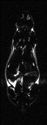
Image Registration. The misalignment of the fat and water signals was corrected using image registration. The exact shift depends on the combination of the off-resonance frequency of fat, receiver bandwidth (as shown in Eq. (2)), and macroscopic Bo field inhomogeneities. The fat-water shift varies spatially, at least in theory. However, we found that bulk fat-water shift due to limited readout bandwidth was the dominant cause of misalignment. We therefore compared the theoretical bulk shift to image registration of the estimated fat and water spin density images. Our initial estimate of the spatial fat water shift (Δx) comes from the scanner’s reported bandwidth and on-resonance frequency, which are recorded in DICOM tags. We used a receiver bandwidth of 220 Hz/voxel in acquiring all images, which gave a theoretical shift of 2.36 pixels. We found the optimal shift by computing mutual information between the estimated fat and water spin density images (Eq. (3), (4)) at offsets from +Δx to –Δx pixels by 0.01 pixel steps (Fig. 1-a). Linear interpolation was used, and a special CV-LIN correction was applied to prevent so-called “scalloping” artifacts (32). Air pixels, as identified in label images described below, were not considered in calculations. We validated that the chemical shift artifact was due to the off-resonance frequency of fat, not field inhomogeneities. The maximum mutual information occurred at the theoretical value of +Δx pixels. It was too slow to repeat the complete search for every dataset; instead the mutual information was calculated only for the theoretical values of +Δx and –Δx from Eq. (2). The offset with the higher mutual information was retained and used for a more accurate and slower piecewise cubic Hermite interpolation before recalculating the ratio image (33). After applying Eq. (6), a corrected ratio image (Fig. 1-c) has sharper edges, clearer intramuscular fat streaks, and a better delineation of the abdominal wall than that before alignment (Fig. 1-b).
a)
b)
c)
Figure 1. Alignment of the fat-only and water-only signals along the frequency encoding direction restores edges lost to the chemical shift artifact. CV-LIN helps to estimate optimal alignment based on mutual information (a). A large ‘scalloping’ artifact appears around whole integer shifts when linear interpolation is used (a, blue dashed line). The use of CV-LIN removes the artifact (a, green solid line), and the optimal solution becomes apparent at the maximum mutual information. The prediction of the optimal alignment from the MRI equations is shown (a, vertical red bars). Visual inspection confirms the prediction of mutual information. The aligned ratio image (c, +2.36 pixel shift) is superior to the unaligned ratio image (b, no shift). Edges at adipose tissue/muscle boundaries are restored around the abdominal wall, and intramuscular fat depots become more apparent.
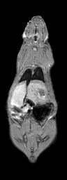
Semi-automatic Image Segmentation. We expedited the measurement of visceral and subcutaneous adipose tissue by automating it as much as possible. The only manual input was tracing the abdominal cavity in all slices of the water-suppressed dataset using Analyze (AnalyzeDirect, Inc., Overland Park, KS). The segmentation was saved as a label image with regions inside and outside the abdominal wall, which was used later to separate visceral and subcutaneous adipose tissue, respectively. Respiratory motion ghosting artifacts and background noise / air were automatically eliminated by creating a mask image using an in-house Matlab program (The Mathworks Inc., Novi, MI) (Fig. 2). Four averages were taken in the image acquisition, effectively reducing the ghost signal intensities. Air voxels were removed from all images by measuring the mean and standard deviation of a 10 pixel x 10 pixel background region in a water-only image (Fig. 2-c). A global lower bound threshold (μ+3σ) was applied to remove air in all slices. This threshold also had the effect of thresholding out some of the weaker ghost artifacts (Fig. 2-d). Remaining air artifacts were removed using the observation that they tended to occur in random positions between slices. We used a 3D morphological opening on each slice with a 2x2x2 structural element to remove small islands of voxels outside the animal. A morphological closing operation with a 2x2x2 structural element removed small holes inside the animals (Fig. 2-e). In some instances, there were remaining air artifacts. The body of the rodent was segmented using region growing and any unconnected voxels were deemed to be air. (Fig. 2-f). In some limited cases it was necessary to manually fix remaining artifacts (Fig. 2-g). Flood fill algorithms are an alternative approach to fixing holes in the mask images, but we found that a simple manual correction was quick and sufficient. At this point, three regions can be identified: external air, interior to the abdominal wall, and exterior to the abdominal wall.
a)
b)

c)

d)

e)

f)

g)
h)
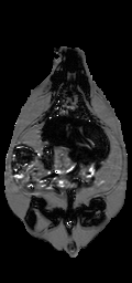
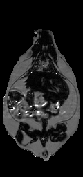
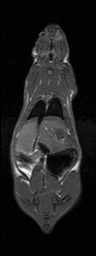
Figure 2. Semi-automatic image processing is used to create a mask. The (fat+water) (a) and fat-only images are transformed into estimates of fat-only and water-only signals as per Eq. 3 and 4 (b, c, resp.). The water-only signal is thresholded to remove air (d). Ghosting artifacts are substantially reduced following morphological opening and closing (e). Disconnected ghosts of high signal are removed by a region growing seeded from the center pixel of the image volume (f). A human observer edits the image map to fix any remaining problems (g). Finally, the mask is applied to the water only signal to show how artifacts have been removed (h).
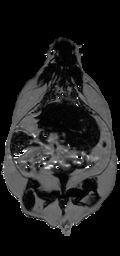
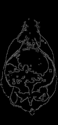
Ratio images were used to identify adipose tissue using a fixed threshold (see below) or, optionally, a user defined threshold. Voxels above the threshold were labeled adipose tissue in the ratio image (Fig. 3-a). Voxels inside and outside the abdominal cavity were labeled as visceral or subcutaneous adipose tissue, respectively. In some limited cases it was necessary to manually remove the interior of bones which have a high fat content and can be misclassified. However, in the majority of cases the bones were significantly smaller than the image resolution. Bright spots in the gastrointestinal tract were eliminated by excluding all voxels in the ratio image with values > 1.0. These bright spots were likely due to peristalsis and/or fecal matter containing iron or copper residues from commercial animal chow. At this point, we have label images consisting of air; visceral adipose tissue; subcutaneous adipose tissue, including some intramuscular fat streaks; muscles/organs inside the abdominal cavity, and muscles/organs outside the abdominal cavity (Fig. 3-b). Volumes were computed without partial volume correction by counting the number of voxels in each label and multiplying by the volume of a single voxel in ml. Volumes were computed with partial volume correction as described later.
a)

b)
c)
Figure 3. Creation of a label image is used by classification and partial volume correction, shown here in a genetically obese SHROB. The ratio image (a) is classified into four classes showed in (b): subcutaneous adipose tissue (white), and visceral adipose tissue (dark gray), muscle/non-adipose tissues (light gray), and air (black). Partial volume correction is performed both on subcutaneous and visceral adipose tissue separately by finding voxels at the boundaries of tissues. The voxels of (b) affected by 3x3 erosion and dilation are labeled for adipose tissue partial volume correction as shown in (c). An alternative is to correct all the pixels in the rat. The arrow indicates a location where intramuscular fat streaks appear but lack strong edges.
Histograms of ratio values were analyzed to find an optimal threshold for separating adipose tissues from muscles and other organs. Peaks in the ratio histograms were found to be remarkably similar between animals. Gaussians fit to the water and fat peaks had means and standard deviations of 0.05±0.02 and 0.77±0.02, respectively. These distributions were comparable to those in an oil/water phantom (see Results, Fig. 4). We used a fixed threshold halfway between the peaks at 0.61.
Partial Volume Correction. Partial volume errors were corrected two different ways. In the first method, we identified and corrected edge voxels. A border of edge voxels were found by computing the difference between dilation and erosion (3x3 structuring element) of the visceral and subcutaneous adipose labels (Fig. 3-c). The signal intensity of each voxel in the ratio image (IR) was modeled as a linear combination weighted by the fraction of adipose tissue in a given voxel (α).
(8)
Where IW and IAT were signal intensities for pure voxels as obtained from the means of Gaussian fits to peaks in the ratio histogram. For the edge voxels, the fraction of adipose tissue (α) was estimated from Eq. 6 using measured IR values. Volume fractions α and (1 - α) in each edge voxel were added to the volume of adipose tissue and muscle/organs, respectively. The α fraction was added to the visceral or subcutaneous volume depending upon whether the edge voxel was originally inside or outside the abdominal cavity, respectively. The (1 - α) fraction was added to the muscle/organs independent of the abdominal cavity. In the second method, we corrected all voxels in the animal using the same algorithm. This was advantageous for unmixing partial volumes due to thick slices.
Signal Intensity Comparison. A single operator placed ROI’s of 5x5 pixels in 3 consecutive slices of the right side of the liver in the ratio images. For comparison ROI’s were also placed in the most uniform regions of muscle in the lower right hindlimb, visceral adipose tissue, and the kidneys. The pixel values were tested for statistically significant differences between lean SHRs, dietary obese SHRs, and genetically obese SHROBs.
Volume Rendering. Because the bias field was removed, ratio images were useful for volume rendering. Volume rendering revealed fat distribution within the animals and was especially useful for identifying fat streaks in the muscle. Ratio images were visualized using a special network script written for volume rendering in Amira (Mercury Computer Systems, Berlin, Germany). Each of the three classes in the label volume was exported separately from Matlab as a series of TIFF files containing the fraction of adipose tissue (α) of 0-1 linearly rescaled to the TIFF range of 1-216 before importing into Amira. Each series of TIFF’s corresponded to separate volumes for muscles/organs, visceral adipose tissue, and subcutaneous adipose tissue. We linked separate color maps and opacity modules to each image volume for rendering. Color maps were customized to provide contrast between tissues (e.g. different shades of pink for subcutaneous and visceral adipose tissue). Opacity was also adjusted to make muscle more opaque than adipose tissues. Rats were viewed from arbitrary angles using camera rotation and cropping. Adipose tissue distribution and partial volume effects were examined. Intramuscular fat streaks of the rats were compared visually.
RESULTS
Ratio Images and Bias Field Correction
Voxel composition, as determined by the ratio model (Eq. (6)), was found to be linear in a phantom of soybean oil and deionized water (Fig. 4-a). Reference signal intensities in the ratio image of water and oil were measured by placing circular ROIs in the image far away from the meniscus. The line profile from pure water to pure oil showed a transition from water (0.05 ± 0.03) to oil (0.75 ± 0.03), which matched the values in the respective ROIs. Ringing artifacts occurred due to limited phase encoding, but a least squares linear regression of signal intensity vs. distance along the line profile was linear with an excellent fit (R2=0.96, Fig. 4-b). This distance was directly proportional to the partial volume effect (α, Eq. (8)) because the line profile was positioned around the exact beginning and end of the intersection of the meniscus with the image grid.
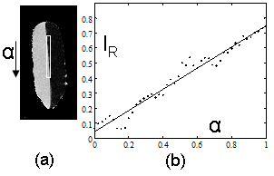
Figure 4. Calibration of ratio calculation on a vegetable oil and deionized water phantom. A line profile (shown as a box in (a)) in a single sagittal slice of the phantom provides a calibration between all-oil and all-water voxels when plotted from top to bottom of the image (b). A linear fit of the data gave IR=0.75*α+0.05(1-α) with R2=0.96 (P<0.01). Oil and water and signal intensities in the ratio image were 0.75±0.03 and 0.05±0.03, respectively.
Signal intensities in the liver varied greatly between cohorts, and some SHROBS exhibited elevated values consistent with hepatic steatosis, a known disease of this rodent model (26) (Fig 5). Lean SHRs had low values (0.01 - 0.04). SHR-DO had slightly higher values (0.03 - 0.08). SHROBs tended to cluster at high (0.12 - 0.24) or low (0.04 - 0.07) liver values, suggesting two phenotypes (SHROB and SHROB*, respectively). As compared to SHROB, the six SHROB* animals had significantly different liver signal intensities (P<0.05). They were not significantly heavier (504.8±46.9 g vs. 438.9±47.3 g, P>0.20) or younger (172.3±28.7 days vs. 201.8±30.8 days, P>0.98). However, they did have more visceral adipose tissue (107.3±16.5 vs. 87.8±3.7 ml, P<0.02). Liver signal intensities in the ratio images were statistically significantly different between all groups (SHR-SHROB, SHR-SHR-DO, SHROB*-SHROB, etc.), except SHROB and SHR-DO (P<0.01). In other tissues, signal intensities in ratio images were very consistent between all animal groups. Muscle, kidney, and visceral adipose tissue signal intensities were not different, and they generally were very flat across images. Intramuscular adipose tissue appeared in both SHROB and SHR-DO, but rarely in lean SHRs.
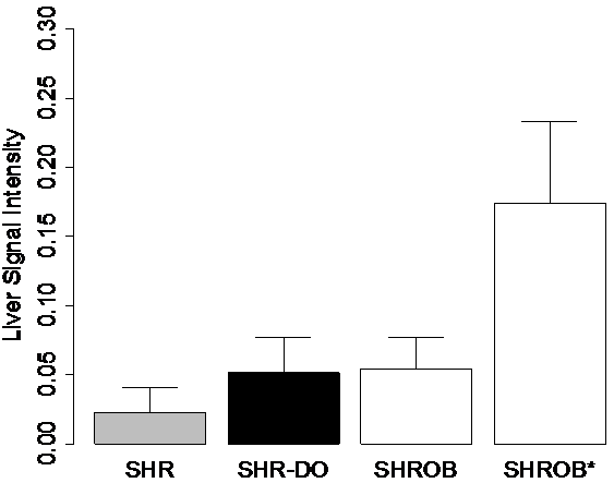
Figure 5. Signal intensities in the liver were consistent with hepatic steatosis, a known disease of this rodent model. ROIs of 5x5 pixels were placed in 3 consecutive slices in each animal in the right side of the liver. Six of the twelve SHROBs (denoted SHROB*) were retrospectively identified as having unusually hyperintense livers. As compared to the other SHROBs, the six SHROB* were not statistically significantly heavier or younger, however they did have more visceral adipose tissue. Signal intensities in the ratio images were statistically significantly different between all groups except SHROB and SHR-DO (P<0.01). Signal intensities in muscle, kidney, and visceral adipose tissue were not different.
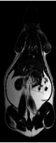
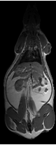
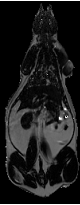
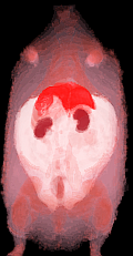
This methodology eliminated a large bias field created by a two-channel phased array coil with one array disabled. The left side of the image was over 200% higher than on the right side in both the fat only image (Fig. 6-a) and fat+water image (Fig. 6-b) of a SHR-DO. This shared left-right bias field was cancelled in the ratio image (Fig. 6-c). The edges of the image were preserved and even enhanced by the elimination of the chemical shift artifact. The contrast of the abdominal wall was improved with respect to adjacent adipose tissues especially on the left side of the image. Substantial signal was recovered in the other regions of the image despite severe coil sensitivity drop-off. Volume rendering in a SHROB was greatly aided by the ratio imaging, which eliminates this type of bias field (Fig. 6-d).
a)
b)
c)
d)
Figure 6. Taking the ratio can also recover datasets which would be otherwise unusable due to coil sensitivity inhomogeneity (a, fat only image and b, fat+water image). Using our method, the 200% left-right bias field in both of the original images is canceled in the ratio image (c). Furthermore, the edges of the abdominal wall are retained. Volume rendering (d) aids in the interpretation of the different amounts of partial volume effects in each type of rat. This SHROB (d) is labeled with color maps for the liver, kidneys, adipose tissue, and other tissues. The ratio values were used for opacity.
Reproducibility of Measurements and Partial Volume Corrections
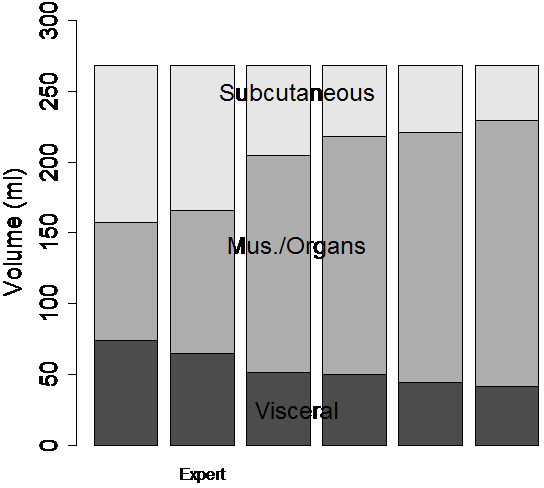
Image analysis variability was reduced by the semi-automatic ratio image analysis program (Fig. 7). Tracings of the abdominal cavity were similar between operators with DSC’s of 0.89, 0.91, 0.93, 0.93, and 0.93. Moreover, the final effect of border delineation on adipose tissue volumes is even less because some regions far from adipose tissue borders will not contribute anyway (see below). The thresholds chosen by the operators in the T1W images caused a disagreement about the classification of adipose tissue voxels, as indicated by DSC’s after thresholding of 0.76, 0.79, 0.81, 0.86, and 0.91. The different thresholds also caused widely varying measurements of visceral and subcutaneous adipose tissue volume, 54.4±12.6 ml and 68.7±30.6 ml, respectively (Fig. 7-a).
a)
b)
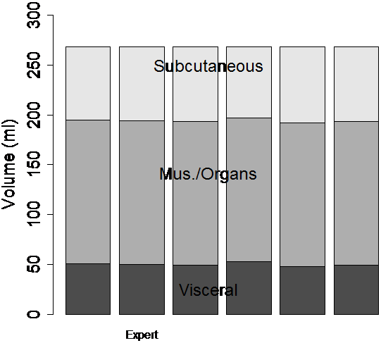
Figure 7. The semi-automatic segmentation was repeated by several human observers on the same data set of a dietary obese SHR (see Fig. 6). Each observer segmented the abdominal cavity independently. When the volumes of the image were computed by thresholding the T1W image, significantly different volumes were measured by each operator (a). After ratio image calculation and partial volume correction of all pixels in the rat, the differences between observers were substantially reduced (b).
When the semi-automatic ratio image analysis program was run using each of the operator’s tracings, the volume measurements became much more consistent (Fig. 7-b). DSC’s improved to 0.96, 0.96, 0.98, 0.98, and 0.99 before applying partial volume correction. Applying partial volume correction on edge voxels gave <1% volume change for each of the 6 analysis volumes. Visceral adipose tissue was 43.9±1.5 ml or 44.0±1.4 ml if only edges were corrected. Subcutaneous adipose tissue was 60.1±1.5 ml before any corrections or 60.6±1.4 ml if only edges were corrected. When we applied partial volume correction to all voxels, the distribution of the 6 measured volumes narrowed and the mean of the 5 moved closer to the expert’s values. That is, because measurements of visceral and subcutaneous adipose tissue volume became more narrowly distributed, 50.1±1.9 ml and 75.2±1.9 ml, respectively after this correction was applied.
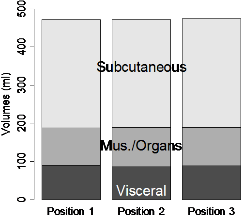
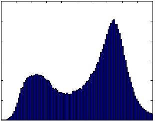
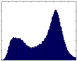
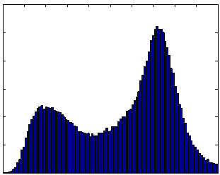
The scan-rescan experiment demonstrated excellent reproducibility and accuracy. When the semi-automated ratio image analysis was used with partial volume correction of all voxels in the rat, measurements of visceral and subcutaneous adipose tissue volumes were remarkably uniform. Visceral adipose tissue volume was 91.2, 87.8, and 90.4 ml for the three measurements, and subcutaneous adipose tissue was 291.1, 288.8, 290.6 ml. Volume measurements of both visceral and subcutaneous adipose tissue were not different, as indicated by the narrow coefficients of variation (i.e. standard deviation divided by mean) of visceral and subcutaneous adipose tissue (2% and 0.5%, respectively). The total volume of the rat was also very reproducible, 472.5, 472.7, and 474.2 ml (Fig. 8-a). The histograms of each of the positions were practically indistinguishable (Fig. 8 b-d). We compared the MRI volumes to the weight of the animal on an electronic scale to determine accuracy. Using a standard density for adipose tissue (0.92 g/ml) and other tissues (1.04 g/ml) (15,34), we converted the MRI volumes to weights of 445.5, 446.4, and 447.4 g. These are very close to the actual body weight determined gravimetrically, 441.7 g. By contrast, a similar analysis prior to partial volume correction of all voxels in the rat produced animal weight estimates of 400.9, 400.5, and 400.5 g, respectively. However, it should be noted that this approximation overestimates total body weight because the volume of the lungs was not excluded. Also, the tail was outside the field of view, so its contribution is not included in the MRI estimates.
a)
b)
c)
d)
Figure 8. Repositioning a SHROB thrice shows remarkably consistent measures of adipose tissue volumes with a standard error <1% of body volume. Despite physically repositioning the rat on the MRI bed and reshimming the scanner, the tissue volumes (a) and histograms (b-d) varied little. Partial volume correction was performed on all pixels in the rat. The total volume of the animal (the top of the subcutaneous adipose tissue bar) was practically invariant between the scans. Tissue volumes measured in the positions were not significantly different (P > 0.50).
We next analyzed partial volume corrections for all rats using abdominal wall tracings from the single expert operator. Corrections were significant for all rats (Fig. 9). Partial volume corrections increased visceral adipose tissue volume by 23±2% (SHR), 15±2% (SHR-DO), 12±1% (SHROB) as a percentage of the total volume of visceral adipose tissue. Likewise, average partial volume correction of subcutaneous adipose tissue volumes increased by 26±1% (SHR), 22±2% (SHR-DO), and 13±1% (SHROB). Since the nominal fat volumes varied greatly between lean SHR and SHROB, these corrections varied from 2.3 to 40.7 ml. If we correct just the edge voxels, changes range from 0.2% to 1% of adipose depot volume for these same data sets. Fig. 3-c shows the location of edge voxels in a SHROB. The biggest relative corrections were in the leaner animals, where muscle and other organs were overestimated in the initial binary segmentation. Generally, most corrections came from intramuscular adipose tissue and as a result of the relatively large slice thickness.
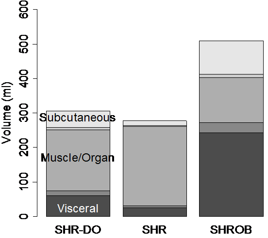
Figure 9. Partial volume corrections differ between types of rats due to the differing adipose distribution. If only the edge pixels are corrected then the overall change in volumes is <1%. However, we found that correcting all the voxels in the rat was significant. The bar plots show each of the depots in ml vs. diet and genetics. The partial volume corrections are shown as gray bars in between the muscle/organ depot and the adipose tissue depots. Generally the amount of correction is proportional to the animal size. The muscle/subcutaneous partial volume effect is smaller in absolute volume, but it is quite large relative to the size of the subcutaneous depot. Partial volume correction enhances the statistical conclusions as described in the text. In every case it was found that the muscle and other organs were over-estimated before partial volume correction.
Genetic/Dietary Obesity Phenotypes
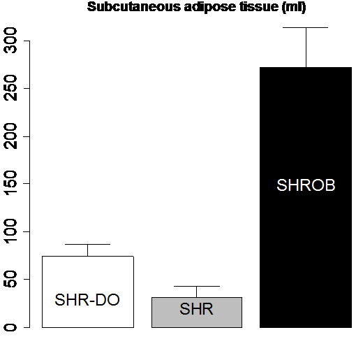
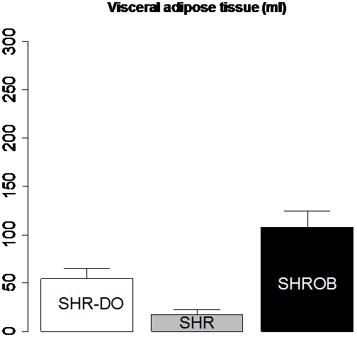
Body composition was very different between lean SHR, and dietary and genetically obese animals (Fig. 10). Subcutaneous adipose tissue volumes (Fig. 10-a) were 278.2±42.4 ml (SHROB), 77.3±13.0 ml (SHR-DO), and 33.0±12.6 ml (SHR). Visceral adipose tissue volumes (Fig. 10-b) were 110.3±17.0 ml (SHROB), 55.9±10.7 ml (SHR-DO), 18.2±5.5 ml (SHR). Subcutaneous adipose tissue volumes were not significantly higher in dietary obesity (P<0.07 SHR-DO vs. SHR) but were highly significantly greater in genetic obesity (P<0.01 SHROB vs. SHR). Visceral adipose tissue volumes were significantly higher in both dietary and genetic obesity (P<0.01 SHR-DO vs. SHR, and P<0.01 SHROB vs. SHR). All differences were several fold greater than the variations measured from the reproducibility measurements above.
a)
b)
Figure 10. Adipose tissue volumes measured by MRI demonstrate differences in body composition with partial volume correction. The genetic obese SHROB rats (N=12) have significantly higher volumes of visceral (b) and subcutaneous adipose tissue (a) than the dietary obese SHR (N=6) and the lean control SHR rats (N=6). The dietary obese SHR have a significantly higher volume of visceral adipose tissue than the lean control. Subcutaneous adipose tissue was not higher in dietary obese SHR as compared to SHR with or without partial volume correction (P<0.10). Error bars indicate one standard deviation. In all cases the error in the measurement are less than the biological variation, which is much less than the underlying genetic and dietary differences.
Biological and dietary variability was found to be much larger than the measurement errors. For example, the SHROB subcutaneous adipose tissue volume was on average 245.2 ml larger than SHR subcutaneous adipose tissue volume. In comparison, the effect of applying partial volume correction was much smaller (2.7-4.6 ml in SHR, 22.0-40.7 ml in SHROB). Intra-operator variability and repositioning had much smaller effects, as measured by our other methods (1.9 ml and <1 ml, respectively). We concluded that the differences we observed reflect underlying biological differences. It would be interesting to investigate the effects of age and sex in a larger study.
Intramuscular adipose tissue was clearly manifested in the ratio images, and 3D volume visualization aided in locating small “streaks.” Volume rendering was useful for visual inspection of fat distribution and the partial volume effect in the rats (Fig. 6-d). It was possible to get an approximate idea of where the fat is stored by interactive cropping and rotating the volume. Whereas lean rats have small amounts of fat stored all throughout their bodies, genetically obese animals have large, solid fat stores in their enlarged adipose tissue depots.
DISCUSSION
The ratio image methodology gives a robust, precise measurement of subcutaneous and visceral adipose tissue volumes. Effectively, it allowed us to remove the bias field due to coil sensitivity inhomogeneity and create a robust image analysis approach. In addition, the ratio technique eliminates additional artifacts such as chemical shift misalignment and partial volumes. Providing an estimate of lipid content is an additional bonus. The technique is sufficiently robust that we believe it could be applied robustly across different animals, scanners, coils, and other external factors.
We simplified the ratio image model with assumptions which are valid under our imaging conditions. We assumed that B0 inhomogeneities were negligible over the rat. Chemical shift-selective excitation techniques are all vulnerable to variations of the main magnetic field, which results in inaccuracies such as incomplete water suppression. Accurate shimming reduces overall B0 variation mitigating the effects of B0 inhomogeneities. The rat and small phantoms we used are far smaller (<20 cm) than uniform portion of the main field in a clinical scanner (30-40cm), which justifies our assumption. Observed data support this conclusion. As an example, typical ratio image values in water of the phantom were 0.01 – 0.05, indicating excellent water suppression. Poor water suppression would give much higher values (e.g. 0.20 – 0.50) and obvious variations in ratio image values across the image. We also neglected RF inhomogeneities (B1 variation). This is justified by the use of the human head coil for transmit in the animal studies, which is again larger than the rats. These are all reasonable assumptions under our imaging conditions on a clinical scanner. However, these assumptions would likely be violated in imaging larger animals and humans, which is where a Dixon-like technique with a B0 map would be more appropriate.
We tested the sensitivity of the model to small changes in the relaxivity parameters to ensure the results did not vary widely. We reprocessed one SHROB dataset with a variation of +10% to -10% in T1W, T2W, T1F, and T2F, and we recomputed tissue volumes and ratio image signal intensities. Subcutaneous adipose tissue volume varied from 273.9 to 276.0 ml, less than a 1% change. Visceral adipose tissue volume varied from 93.9 to 96.6 ml, only a 3% change. Muscle/organ volume varied from 117.8 to 122.7 ml, less than a 4% change. The mean signal intensity in the ratio images from 0.78 to 0.81 in visceral adipose tissue, 0.06 to 0.07 in muscle, 0.04 to 0.05 in kidneys, and 0.06 to 0.07 in liver. These signal intensity variations were as small as the variations in the ratio images using the initial relaxivities (e.g. 0.02 standard deviation in liver). We concluded that the model produced consistent results. We assumed that our choice of fat and water relaxivities was adequate for our imaging conditions. This is justified by the short TE, which made the sequence insensitive to T2. Our acquisitions were also somewhat desensitized to T1 by the long TR (i.e. 1200 ms).
An alternative to assuming constant relaxivities is to estimate them from MR measurements on a voxel or tissue basis. A relaxometry experiment could be designed to estimate T1 and T2 for each voxel by acquiring multiple echo times and multiple repetition times. Assuming that water and fat are the dominant proton species in each voxel, estimated values could be used in the calculation of the ratio image, Eq. (6). Related corrections have been implemented in Iterative Decomposition of water and fat with Echo Asymmetry and Least squares estimation (IDEAL). Liu et al. developed a per-voxel T1 correction based on dual flip angles at the cost of doubling the number of scans required (35). Yu et al. presented a per-voxel T2* correction where the T2* of both fat and water were assumed to be equal due to an injection of Feridex (36). At least in human imaging, iron accumulation in the liver can be a confound for lipid measurements due to T2* effects (37), which suggests that estimation of relaxometry parameters is required for accurate quantitation. However, voxel estimation of T1 and T2 will necessarily be noisy and depend upon MR artifacts. Ideally, partial volume effects should be considered, but these are rarely modeled in T1 and T2 mapping. T1 maps are a potential alternative to the ratio technique described here. However, while T1 mapping could be a useful tool for measuring adipose tissue volumes, this technique may show difficulties when used for intravoxel lipid levels as the T1 of water varies significantly from tissue to tissue. Therefore, knowledge of the T1 of the water in each tissue (e.g. liver and muscle) would be needed to determine a fat fraction in each of these tissues. Our method should be less sensitive to the effects of iron due to the dependence on T2, not T2*. We would not expect a significant variation in liver iron content in these in-bred rats eating controlled diets, but there are situations where the T2 of water protons in the liver could vary from subject to subject. Clark et al. demonstrated significant T2 variations among patients with inherited diseases resulting in iron-overloaded livers (38). Using average tissue values remains a viable alternative, especially when sensitivities to relaxometry parameters are minimal as argued above.
Our method might not be applicable to high field scanners. At higher field strengths typical for small animal imaging research studies, several artifacts become worse such as B0 inhomogeneities and chemical shift artifacts. This model can still fix the chemical shift between fat and water, which increases in both Hz and pixels at high field strength. The maximum read-out bandwidth is constrained by gradient strength and the ADC sampling rate, which may be a limiting factor on some scanners but not on preclinical scanners. The tissue relaxitivites change, but T1 and T2 variations can be incorporated into this model with reasonable estimates. The model can also be adapted to a wide variety of pulse sequences / parameters (i.e., FLASH vs. Spin Echo, TR/TE, flip angle, etc.). As it is derived, the model cannot compensate B1 variation, B0 inhomogeneity, or eddy currents, which are problematic on higher field MRI systems. Fortunately, these types of errors could potentially be compensated for directly with MR acquisition techniques such as adiabatic RF excitation pulses to limit B1 heterogeneity or the use of the multi-point Dixon techniques to correct for Bo inhomogeneities.
In its present implementation, a downside is the requirement for two image acquisitions which essentially doubles the overall acquisition time. However, multiple gradient echo acquisitions (39) or alternative trajectories (40) approaches can be utilized to reduce the acquisition time closer to a single acquisition. Another advantage of a multiple gradient echo acquisition is that fat and water can be separated by modeling the fat-water phase differences. Additional proton species can be resolved if their frequency offsets are known, which would be useful for estimating the chemically unsaturated proton species. Another approach is to obtain a single water-suppressed image and correct any bias field inhomogentity prior to quantifying fat volumes. One approach is to fit a low-order polynomial to the image and correct the bias field by minimizing image entropy (41,42). Some studies have not corrected the bias field at all (19,21,43). But, as we have shown here at 1.5T, these effects can be quite significant and can result in lipid quantitation errors as the thresholding/segmentation processes become inaccurate or unreliable.
The three groups of rats provide an interesting contrast between genetic and dietary obesity. Genetically obese SHROBs have a number of metabolic diseases, including severe insulin resistance, glucose intolerance, and hyperlipidemia (44). We found that SHROBs have six times as much visceral adipose tissue and eight times as much subcutaneous adipose tissue as lean control SHRs. In contrast, dietary obese animals (SHR-DOs) have three times the visceral adipose tissue but only twice the subcutaneous adipose tissue of lean control SHRs, and the difference in subcutaneous adipose tissue is not statistically significant. Apparently both diet and genetics are correlated with visceral obesity, but massive expansion of the subcutaneous depot is unique to genetic obesity. Visceral adipose tissue is strongly correlated with metabolic diseases, especially insulin resistance (45). Insulin resistance is apparent in SHROBs with fasting insulin increased to at least 10 times that of SHR littermates while fasting glucose is unchanged (28). Glucose to insulin ratio, an index of insulin resistance, is 9-fold higher in SHROB than SHR. Dietary obese, SHR-DO, animals were comparably insulin resistant to the SHROB animals (9). The increased insulin resistance in the SHR-DO animals correlates well with the increases in visceral depots, which reinforces the link between visceral obesity and insulin resistance (46). It remains an open question whether subcutaneous adipose tissue is an independent predictor of insulin resistance, but some preliminary studies in humans support this hypothesis (8,47). Bergman et al. observe that metabolic damage and insulin resistance are caused by the storage of lipids outside of visceral adipose tissue (48). The phenotype of SHROBs with elevated visceral adipose tissue and liver fat content is consistent with this “lipid overflow hypothesis.” Briefly, this hypothesis states that if the storage capacity of the adipose tissue is exceeded, fat will be stored in other organs (i.e. ectopic fat depots such as liver). This is thought to cause deleterious effects at its eventual destination (7,49). Our data support the hypothesis because the genetically obese SHROBs have tremendously enlarged adipose depots with fat accumulation in the liver, which may indicate that they exceeded the limit of fat storage in their adipose tissues. In contrast, the lean rats do not seem to have reached the limit because they do not have fat accumulation in the liver, and their adipose depots are normal or only slightly enlarged. The most interesting aspect of our rat model is that the dietary obese rats have a selectively enlarged visceral adipose tissue depot and slightly elevated liver fat, which suggests that diet should be considered a factor in this hypothesis.
The results we have shown here demonstrate the importance of partial volume correction for measuring adipose tissue volumes. The primary motivation for partial volume correction in this study was to increase accuracy as well as precision. Voxel anisotropy caused partial volumes to occur because the slices were thicker than the in-plane voxel size. This motivates a partial volume correction to make the data from different animals comparable. The images were acquired at different resolutions due to the different sizes of the animals and constraints of using a clinical scanner. Therefore we corrected partial volume effects in every pixel of the rat to remove this source of variability. It is not surprising that the volumes differ depending on whether all the voxels or just edge voxels were corrected because correcting only the edge voxels leaves a binary segmentation in all non-edge voxels. Alternatives include post-processing corrections, such as Gaussian mixture models and interpolation with reverse diffusion (50).
We have also identified a robust method for calibrating lipid concentration. There are a variety of methods in the literature. Oil-water emulsions are commonly used to make a series of phantoms, but it is difficult to make a stable emulsion over a wide range of oil concentration with the same surfactant, owing to the challenge of stabilize both oil-in-water and water-in-oil emulsions (18). Further, these emulsions may precipitate (i.e. break down) over time, which would undermine the reproducibility of a longitudinal study. We chose an alternative approach based on manipulating the partial volume effect. The image acquisition of an unmixed oil-water phantom can be varied to create partial volumes, recreating the portioning of the biological specimen into fat and lean compartments. A thick slice can be shifted across the oil-water meniscus, but this requires many scans (51). Another alterative is to make non-selective projections of oil-water ‘wedge’ phantoms on the frequency encoding axis, but this requires a custom image reconstruction (52). This has proven to be a robust technique which we believe is appropriate for studies where reproducibility is a concern.
Scan-rescan variation gives a general indication of the magnitude of all instrument errors combined with the variability of physically placing the animal in the scanner over a short time. There may be additional instrument variability over a longitudinal experiment. An important aspect was that the animals were positioned casually, and not positioned according to landmarks or placed in a molded frame to lock position. Also, the obese animals were considerably more difficult to position. Our scan-rescan-rescan repositioning experiment showed that the total volume of the rat varied <1.0 ml, which indicates the insensitivity of the analysis algorithm to positioning. This is an important feature for imaging of deformable rodent models. It should be noted that the same operator processed these datasets, which therefore do not include inter-operator variability.
For rapid comparison of animals, we find volume rendering useful. Volume rendering has previously been used to visualize adipose tissue distribution, which has aided studies of obese rodents. Calderan et al. performed a 3D reconstruction of T1-weighted images, which assisted in interpreting anatomical relationships in obese mice (53). They noted the distribution of adipose tissue in an obese rat was predominantly subcutaneous along the caudal aspect of the animal, and the visceral adipose tissue had displaced one of the kidneys. We have also found volume rendering to be useful for examining intramuscular adipose tissue (i.e. “fat streaks”) as well as distention of the abdominal cavity. Our ratio imaging methodology works extremely well with volume rendering / classification techniques because of the correction of the bias fields. Large bias fields make volume rendering much harder to interpret because the non-uniform intensity causes confusing intensity variation in the volume renderings.
In conclusion, we have developed a robust imaging and analysis paradigm centered on the generation of ratio images to enable effective phenotyping of rodent models of obesity. The remarkable homogeneity of ratio images is useful for both segmentation and 3D visualization, and reproducibility is also improved. The simplicity and reproducibility of this technique is promising for large scale studies of body composition in obese rodents influenced by diet, genetics, exercise, and drugs. These techniques are also generally applicable to clinical research studies of obesity where it is becoming important to quantify regional lipid distribution to track the effects of diet and exercise interventions (54).
References
1. Fontaine KR, Redden DT, Wang C, Westfall AO, Allison DB. Years of Life Lost Due to Obesity. JAMA 2003:289:187-193.
2. Olshansky SJ, Passaro DJ, Hershow RC, et al. A Potential Decline in Life Expectancy in the United States in the 21st Century. N.Engl.J Med. 2005:352:1138-1145.
3. Bouchard C, Johnston FE. Fat Distribution During Growth and Later Health Outcomes, New York, NY: Liss; 1988. 363 p.
4. Bray GA. Pathophysiology of Obesity. Am J Clin Nutr 1992:55:488S-494S.
5. Seidell JC, Bjorntorp P, Sjostrom L, Sannerstedt R, Krotkiewski M, Kvist H. Regional Distribution of Muscle and Fat Mass in Men--New Insight into the Risk of Abdominal Obesity Using Computed Tomography. Int.J Obes. 1989:13:289-303.
6. Matsuzawa Y, Shimomura I, Nakamura T, Keno Y, Kotani K, Tokunaga K. Pathophysiology and Pathogenesis of Visceral Fat Obesity. Obes Res 1995:3 Suppl 2:187S-194S.
7. Yki-Jarvinen H. Ectopic Fat Accumulation: an Important Cause of Insulin Resistance in Humans. J R.Soc.Med. 2002:95 Suppl 42:39-45.
8. Goodpaster BH, Thaete FL, Simoneau JA, Kelley DE. Subcutaneous Abdominal Fat and Thigh Muscle Composition Predict Insulin Sensitivity Independently of Visceral Fat. Diabetes 1997:46:1579-1585.
9. Johnson JL, Wan DP, Koletsky RJ, Ernsberger P. A New Rat Model of Dietary Obesity and Hypertension. Obes Res 2005:13:A113-A114.
10. Johnson DH, Flask CA, Wan DP, Ernsberger PR, Wilson DL. Quantification of Adipose Tissue in a Rodent Model of Obesity. Medical Imaging 2006: Physiology, Function, and Structure from Medical Images. The International Society for Optical Engineering 2-12-2006 San Diego, CA, USA. In: Proc SPIE 6143:2-11.
11. Ishikawa M, Koga K. Measurement of Abdominal Fat by Magnetic Resonance Imaging of OLETF Rats, an Animal Model of NIDDM. Magnetic Resonance Imaging 1998:16:45-53.
12. Tang H, Vasselli JR, Wu EX, Boozer CN, Gallagher D. High-Resolution Magnetic Resonance Imaging Tracks Changes in Organ and Tissue Mass in Obese and Aging Rats. American journal of physiology.Regulatory, integrative and comparative physiology. 2002:282:R890-R899.
13. Tang HY, Vasselli J, Wu E, Gallagher D. In Vivo Determination of Body Composition of Rats Using Magnetic Resonance Imaging. In Vivo Body Composition Studies 2000:904:32-41.
14. Ross R, Leger L, Guardo R, De GJ, Pike BG. Adipose Tissue Volume Measured by Magnetic Resonance Imaging and Computerized Tomography in Rats. J Appl.Physiol 1991:70:2164-2172.
15. Tang H, Vasselli JR, Wu EX, Boozer CN, Gallagher D. High-Resolution Magnetic Resonance Imaging Tracks Changes in Organ and Tissue Mass in Obese and Aging Rats. Am J Physiol Regul.Integr.Comp Physiol 2002:282:R890-R899.
16. Gonzalez Ballester MA, Zisserman AP, Brady M. Estimation of the Partial Volume Effect in MRI. Med.Image Anal. 2002:6:389-405.
17. Zhang X, Tengowski M, Fasulo L, Botts S, Suddarth SA, Johnson GA. Measurement of Fat/Water Ratios in Rat Liver Using 3D Three-Point Dixon MRI. Magn Reson Med 2004:51:697-702.
18. Poon CS, Szumowski J, Plewes DB, Ashby P, Henkelman RM. Fat/Water Quantitation and Differential Relaxation Time Measurement Using Chemical Shift Imaging Technique. Magnetic Resonance Imaging 1989:7:369-382.
19. Schick F, Machann J, Brechtel K, et al. MRI of Muscular Fat. Magnetic Resonance in Medicine 2002:47:720-727.
20. Goodpaster BH, Stenger VA, Boada F, et al. Skeletal Muscle Lipid Concentration Quantified by Magnetic Resonance Imaging. Am J Clin Nutr 2004:79:748-754.
21. Machann J, Bachmann OP, Brechtel K, et al. Lipid Content in the Musculature of the Lower Leg Assessed by Fat Selective MRI: Intra- and Interindividual Differences and Correlation With Anthropometric and Metabolic Data. J Magn Reson Imaging 2003:17:350-357.
22. Lunati E, Marzola P, Nicolato E, Fedrigo M, Villa M, Sbarbati A. In Vivo Quantitative Lipidic Map of Brown Adipose Tissue by Chemical Shift Imaging at 4.7 Tesla. J.Lipid Res. 1999:40:1395-1400.
23. Haase A, Frahm J, Hanicke W, Matthaei D. 1H NMR Chemical Shift Selective (CHESS) Imaging. Physics in Medicine and Biology 1985:30:341-344.
24. Haacke EM, Brown RW, Thompson MR, Venkatesan R. Water/Fat Separation Techniques. In: Haacke EM, Brown RW, Thompson MR, and Venkatesan R, editors. Magnetic resonance imaging : physical principles and sequence design, 1st edition. New York: John Wiley & Sons, Inc.; 1999. p 421-449.
25. Hussain HK, Chenevert TL, Londy FJ, et al. Hepatic Fat Fraction: MR Imaging for Quantitative Measurement and Display--Early Experience. Radiology 2005:237:1048-1055.
26. S Koletsky. New Type of Spontaneously Hypertensive Rats With Hyperlipemia and Endocrine Gland Defects. Spontaneous Hypertension: Its Pathogenesis and Complications 1972:194-197.
27. Grundy SM. Small LDL, Atherogenic Dyslipidemia, and the Metabolic Syndrome. Circulation 1997:95:1-4.
28. Wan DP, Johnson DH, Johnson JL, Koletsky RJ, Flask C, Ernsberger P. Magnetic Resonance Imaging of Visceral and Subcutaneous Fat Distribution in Genetic Versus Dietary Obesity. NAASO 2005 Annual Scientific Meeting. 10-15-2005 Vancouver, Canada. In: NAASO, The Obesity Society, 2005 National Meeting .
29. Iacobellis G. Imaging of Visceral Adipose Tissue: an Emerging Diagnostic Tool and Therapeutic Target. Current drug targets - Cardiovascular & haematological disorders 2005:5:345-353.
30. Dice LR. Measures of the Amount of Ecologic Association Between Species. Ecology 1945:26:297-302.
31. Bartko JJ. Measurement and Reliability: Statistical Thinking Considerations. Schizophr.Bull. 1991:17:483-489.
32. Salvado O, Wilson DL. Removal of Local and Biased Global Maxima in Intensity-Based Registration. Med.Image Anal. 2007:11:183-196.
33. Kahaner D, Moler C, Nash S. Numerical methods and software, Upper Saddle River, NJ, USA: Prentice-Hall, Inc.; 1989. 495 p.
34. Gallagher D, Belmonte D, Deurenberg P, et al. Organ-Tissue Mass Measurement Allows Modeling of REE and Metabolically Active Tissue Mass. Am J Physiol 1998:275:E249-E258.
35. Liu CY, McKenzie CA, Yu H, Brittain JH, Reeder SB. Fat Quantification With IDEAL Gradient Echo Imaging: Correction of Bias From T(1) and Noise. Magn Reson Med 2007:58:354-364.
36. Yu H, McKenzie CA, Shimakawa A, et al. Multiecho Reconstruction for Simultaneous Water-Fat Decomposition and T2* Estimation. J Magn Reson Imaging 2007:26:1153-1161.
37. Westphalen AC, Qayyum A, Yeh BM, et al. Liver Fat: Effect of Hepatic Iron Deposition on Evaluation With Opposed-Phase MR Imaging. Radiology 2007:242:450-455.
38. Clark PR, St Pierre TG. Quantitative Mapping of Transverse Relaxivity (1/T(2)) in Hepatic Iron Overload: a Single Spin-Echo Imaging Methodology. Magn Reson Imaging 2000:18:431-438.
39. Hardy PA, Hinks RS, Tkach JA. Separation of Fat and Water in Fast Spin-Echo MR Imaging With the Three-Point Dixon Technique. J Magn Reson Imaging 1995:5:181-185.
40. Flask CA, Dale B, Lewin JS, Duerk JL. Radial Alternating TE Sequence for Faster Fat Suppression. Magn Reson Med 2003:50:1095-1099.
41. Salvado O, Hillenbrand C, Zhang S, Wilson DL. Method to Correct Intensity Inhomogeneity in MR Images for Atherosclerosis Characterization. IEEE Trans.Med.Imaging 2006:25:539-552.
42. Sled JG, Zijdenbos AP, Evans AC. A Nonparametric Method for Automatic Correction of Intensity Nonuniformity in MRI Data. IEEE Trans.Med.Imaging 1998:17:87-97.
43. Changani KK, Nicholson A, White A, Latcham JK, Reid DG, Clapham JC. A Longitudinal Magnetic Resonance Imaging (MRI) Study of Differences in Abdominal Fat Distribution Between Normal Mice, and Lean Overexpressors of Mitochondrial Uncoupling Protein-3 (UCP-3). Diabetes, Obesity and Metabolism 2003:5:99-105.
44. Ernsberger PR, Koletsky RJ, Friedman JE. Molecular Pathology in the Obese Spontaneous Hypertensive Koletsky Rat: a Model of Syndrome X. Ann.N.Y.Acad.Sci. 1999:892:272-288.
45. Heymsfield SB, Wang Z, Lohman T, Going S. Human Body Composition, 2nd edition. Human Kinetics; 2005. 522 p.
46. Despres JP, Moorjani S, Lupien PJ, Tremblay A, Nadeau A, Bouchard C. Regional Distribution of Body Fat, Plasma Lipoproteins, and Cardiovascular Disease. Arteriosclerosis 1990:10:497-511.
47. Tulloch-Reid MK, Hanson RL, Sebring NG, et al. Both Subcutaneous and Visceral Adipose Tissue Correlate Highly With Insulin Resistance in African Americans. Obes Res 2004:12:1352-1359.
48. Bergman RN, Kim SP, Catalano KJ, et al. Why Visceral Fat Is Bad: Mechanisms of the Metabolic Syndrome. Obes Res 2006:14 Suppl 1:16S-19S.
49. Rasouli N, Molavi B, Elbein SC, Kern PA. Ectopic Fat Accumulation and Metabolic Syndrome. Diabetes Obes Metab 2007:9:1-10.
50. Salvado O, Hillenbrand CM, Wilson DL. Partial Volume Reduction by Interpolation With Reverse Diffusion. International Journal of Biomedical Imaging 2006:2006:1-13.
51. Namimoto T, Yamashita Y, Mitsuzaki K, et al. Adrenal Masses: Quantification of Fat Content With Double-Echo Chemical Shift in-Phase and Opposed-Phase FLASH MR Images for Differentiation of Adrenal Adenomas. Radiology 2001:218:642-646.
52. Brix G, Heiland S, Bellemann ME, Koch T, Lorenz WJ. MR Imaging of Fat-Containing Tissues: Valuation of Two Quantitative Imaging Techniques in Comparison With Localized Proton Spectroscopy. Magn Reson Imaging 1993:11:977-991.
53. Calderan L, Marzola P, Nicolato E, et al. In Vivo Phenotyping of the Ob/Ob Mouse by Magnetic Resonance Imaging and 1H-Magnetic Resonance Spectroscopy. Obes Res 2006:14:405-414.
54. Chan JM, Rimm EB, Colditz GA, Stampfer MJ, Willett WC. Obesity, Fat Distribution, and Weight Gain As Risk Factors for Clinical Diabetes in Men. Diabetes Care 1994:17:961-969.