Uniform Spinning Sampling Gradient Electron Paramagnetic Resonance Imaging
David H. Johnson, Rizwan Ahmad, Yangping Liu, Zhiyu Chen, Alexandre Samouilov, and Jay L. Zweier
This is an author's electronic pre-print of the following publication. MRM allows pre-prints to be shared through individual author's websites; for terms, please see this website's license. Please cite the published work as:
Johnson DH, Ahmad R, Liu Y, Chen Z, Samouilov A, Zweier JL. Uniform spinning sampling gradient electron paramagnetic resonance imaging. Magn Reson Med 2013 Mar. PMID: 23475830. DOI: 10.1002/mrm.24712
Address for correspondence: Jay L. Zweier, MD. jay.zweier@osumc.edu
Running Title: Uniform Spinning Gradient EPRI
Abstract
Purpose: To improve the quality and speed of electron paramagnetic resonance imaging (EPRI) acquisition by combining a uniform sampling distribution with spinning gradient acquisition.
Theory and Methods: A uniform sampling distribution was derived for spinning gradient EPRI acquisition (Uniform Spinning Sampling, USS) and compared to the existing (Equilinear Spinning Sampling, ESS) acquisition strategy. Novel corrections were introduced to reduce artifacts in experimental data.
Results: Simulations demonstrated that USS puts an equal number of projections near each axis whereas ESS puts excessive projections at one axis, wasting acquisition time. Artifact corrections added to the magnetic gradient waveforms reduced noise and correlation between projections. USS images had higher SNR (85.9±0.8 vs. 56.2±0.8) and lower mean-squared error than ESS images. The quality of the USS images did not vary with the magnetic gradient orientation, in contrast to ESS images. The quality of rat heart images was improved using USS compared to that with ESS or traditional fast-scan acquisitions.
Conclusion: A novel EPRI acquisition which combines spinning gradient acquisition with a uniform sampling distribution was developed. This USS spinning gradient acquisition offers superior SNR and reduced artifacts compared to prior methods enabling potential improvements in speed and quality of EPR imaging in biological applications.
Introduction
In vivo electron paramagnetic resonance (EPR) imaging enables spatial mapping of paramagnetic probes in a variety of in vivo and ex vivo biomedical applications (1-3). EPR can quantitate paramagnetic molecules in biological systems with direct measurement of relatively stable free radicals and trapping of labile radicals such as O2-derived superoxide, hydroxyl radicals or NO that are implicated in disease pathogenesis (4-6). Using paramagnetic probes, cellular radical metabolism, redox state, O2, pH, and cell death can be measured (7). EPR is inherently more sensitive than nuclear magnetic resonance because the magnetic moment of the electron is 658 times larger than the proton, and there is negligible background EPR signal in vivo. However, a challenge in performing in vivo EPR imaging experiments is the relatively long acquisition time required. A particularly difficult aspect of this problem is acquiring a sufficient number of projections to resolve the spatial distribution of the probe within the constraints of limited signal to noise ratio and respiratory or cardiac motion. To this end, the spinning magnetic gradient technique was developed to rapidly acquire nearly limitless numbers of projections in a very short amount of time (8,9). It was further extended to 3D acquisitions, but its full potential has yet to be realized.
EPR experiments can be classified as either continuous wave (CW) or time-domain (pulsed) acquisitions. Pulsed EPR experiments have the potential for much faster acquisitions, but the choice of imaging probes is limited to those with longer relaxation times. Also, the resonator design must be adapted to minimize dead time at the expense of other design parameters (e.g., Q and homogeneity). In contrast, CW EPR allows use of a wider variety of probes with simpler synthesis and better in vivo tolerance. For example, nitroxides are well characterized in cardiac EPR experiments (2), and they are readily usable in CW EPR but not pulsed EPR due to their short relaxation times. The focus of this work is on expediting the CW EPR experiment for biological applications.
CW EPR imaging is limited by the signal to noise ratio available during biologically relevant acquisition times. The conventional fast-scan acquisition holds the gradients constant while the main magnetic field is swept, which produces a relatively small number of slower but higher SNR projections and image reconstruction artifacts due to angular undersampling (10). While this technique produces many points in each projection, the acquisition must be repeated for every projection and results in a long total acquisition time. An alternative method is rapid-scan EPR, where the electron signal is directly detected with a very short acquisition time, resulting in more projections and lower SNR in each projection. The spinning magnetic gradient technique is an alternative CW EPR acquisition which holds the main magnetic field constant while the gradients are rotated. The acquisition is repeated for each point in the range of the main magnetic field sweep. This makes a unique tradeoff in acquiring more projections rather than more points in each projection. In fast-scan technique, each projection is sampled above the Nyquist rate by as much as a factor of ten, which results in data redundancy. The spinning gradient technique, on the other hand, allows decreasing the number of points in each sample. When SNR is the limiting experimental factor, the spinning magnetic gradient technique has the potential to utilize the acquisition time more effectively by reducing data redundancy.
A critical limitation of the spinning magnetic gradient technique is the inefficient distribution of projections, which leads to overly dense sampling near the poles of the sphere (11). It has already been well established in non-spinning gradient acquisitions that a uniform distribution of projections over the sphere substantially improves the reconstructed images (12,13). By adapting the concept of uniformly distributing points on the hemisphere to the spinning magnetic gradient technique, we expect to observe a reduction in artifacts and improvements in the signal to noise ratio (SNR) in the reconstructed images. An EPR instrument recently developed in our group provides unique capabilities to achieve this goal by providing low inductance gradients (3), resonators designed specifically for cardiac imaging (14), and fast software specifically written for cardiac gating and 3D visualization (15).
The theory of the spinning magnetic gradient technique was established by Ohno and Watanabe and then refined by Deng et al. (8,9,11). Previously, Equilinear Spinning Sampling (ESS) was used to generate the gradient waveforms for 3D EPR imaging (11). ESS increments the azimuth and elevation angles by constant amounts. While ESS is simple to implement, it does not provide uniform sampling; oversampling occurs at the poles because a constant angular increment fails to account for the Jacobian of the transformation to the surface of a sphere. In this work, we propose a new method, called Uniform Spinning Sampling (USS), which provides nearly uniform distribution of projections for spinning gradient acquisition. USS is based on previous work on generating uniformly distributed points on a sphere (16). Briefly, USS uses an arcsin transformation of the elevation angle, which compensates for oversampling at one of the axes. USS also fixes the ratio of the azimuth and elevation angles to very closely approximate uniform solid angle sampling. Both USS and ESS have a constant analog output clock rate on the gradient waveforms, which make them easy to implement on the same hardware.
Subramanian et al. developed an acquisition that combined spinning gradients with rapid magnetic field scanning and direct detection (17,18). In the rapid scan rotating gradient method both the magnetic gradients and magnetic field are simultaneously oscillated, corresponding to acquiring unique pairs of main magnetic field values and gradient values. The technique is extremely fast because it removes the limitations of low frequency magnetic field modulation and traditional phase sensitive detection. While rapid scan rotating gradients has the promise of very short temporal resolution, many averages are needed for in vivo experiments to compensate for the lowered SNR due to the short sampling time. Specialized digital integration circuits are needed to average the signal, and only 35% of the acquisition time during each half-cycle can be spent acquiring the signal because the driving sine wave is nonlinear in the remaining time. The technique has not yet been demonstrated for 3D or in vivo applications, and additional ringing artifacts must be corrected by deconvolution when high scan rates are used. In contrast, the spinning magnetic gradient technique developed here works with existing EPR hardware without modification and can easily be applied to in vivo experiments.
In this work, we report a modified spinning gradient acquisition that produces an efficient and uniform distribution of projections. We also correct several artifacts that can affect the spinning gradient data, and we address some of the hardware limitations of the technique. Results are demonstrated in both test phantoms and also a biological application in the isolated rat heart.
Theory
For N projections with azimuthal angle θ and elevation angle φ, the components of the gradient vector are defined by:
(1)
where CX, CY, and CZ are calibration constants (11). Both ESS and USS start in the XY plane and spiral upward toward the Z axis by definition in Eq (1). ESS takes the following form:
(2)
R is a free parameter that determines the relative frequencies at which the elevation and azimuthal angles change. The value of R=8 was previously used by Deng et al. independent of N and is used for all ESS experiments in this paper (11).
USS is defined by the following formulas:
(3)
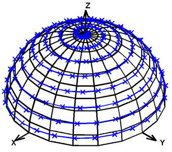
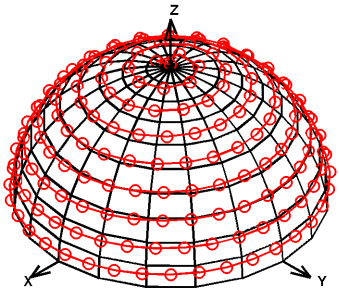
The key difference is the use of the arcsin function to compensate for the excessive number of projections near the Z axis (i.e., when φ approaches π/2). The resulting changes to the distribution of projections are made apparent by visually inspecting their locations on the unit hemisphere (Figure 1). This modification slightly increases the gradient rotation frequency towards the end of each cycle (Figure 2). These changes do not require significant hardware modifications, but the resulting distribution of points on the hemisphere is nearly uniform.
a)
b)
Figure 1. Distribution of 400 projections on the unit hemisphere for Equilinear Spinning Sampling (ESS, a) and Uniform Spinning Sampling (USS, b) shows that ESS puts a disproportionate number of projections near the Z axis (89 projections within 20º of the Z axis, or 22%, as compared to 16 projections near the Y axis, or 4%), whereas USS does not favor any axis or location on the hemisphere (25 projections, or 6%, near each of the X, Y, and Z axes).
Spinning gradient acquisitions are different than conventional EPR imaging acquisitions in that one data point is acquired in every projection at a constant magnetic field before proceeding to the next magnetic field value. In contrast, conventional acquisitions are formed from acquiring a single, complete projection at a time. The spinning gradient data are rearranged to the conventional ordering before the reconstruction is performed. While the reconstruction itself is the same for both types of acquisitions, a key difference between them is that adjacent points in time are correlated in a different way. Each point in the resulting spinning gradient dataset is drawn from a different repetition of the sequence. This motivates the development of the bridge detector current offset (DCO) correction described later in this work.
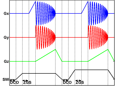
Figure 2. Modified gradient waveforms for the spinning gradient acquisition include two new features: DCO correction and automatic Zero Gradient Spectrum (ZGS) acquisition. An additional amount of time is spent with the gradients turned off to correct the unstable DCO level and also acquire a ZGS at the same field shift as the projection data.
Methods
A home-built L-band EPR imaging system operating at 1.2 GHz was used to record projections using both the ESS and USS acquisitions (3). This system has low inductance gradient coils (85 μH for X and Y, 67 μH for Z) and a sweep coil that can be swept from 5 to 400 mT in under 10 seconds, which enables fast changes in the gradients and sweep field. The previously reported fast-scan acquisition was also performed for comparison (12).
A resolution assessment phantom was constructed from three 100 µl capillary tubes each containing approximately 5 mg lithium phthalocyanine (LiPc), purged with Argon gas and then flame sealed. The capillaries were inserted into slots separated by 5 mm in a 20 mm diameter Rexolite cylinder. This probe was chosen for its single, sharp peak and stability, which enabled fair comparisons between the different types of acquisitions. ESS and USS images were acquired with 1,024 projections in 64 seconds, 64 points per projection, 25 mT/m gradient amplitude over a 60 mm field of view, 45 mT center field, 1.5 mT sweep width, 0.089 mT modulation amplitude, and 100 KHz modulation frequency. A high SNR reference fast-scan image was acquired with 3,600 projections acquired in 21 minutes and 1,024 points per projection. The other parameters were the same.
A male Sprague-Dawley rat (300-350 g) was anesthetized with pentobarbital (60 mg/kg) and heparinized (0.1 ml of 1000 IU/kg) via intraperitoneal injection. Under deep anesthesia the heart was excised, and the aorta was cannulated. The heart was perfused in a retrograde Langendorff mode under constant pressure of 80 mmHg with phosphate buffered saline (PBS) containing 100 µM CaCl2. After washing out the blood, the perfusion line was switched to an infusion line. The EPR probe solution used consisted of paramagnetic nanoparticles which were prepared by adding a solution of lithium octa-n-butoxynaphthalocyanine (LiNc-BuO, 20 mg) (19) and lecithin (140 mg) in THF (1 mL) into 10 mL of a fast stirred PBS, followed by removal of the organic solvent under vacuo. Five ml of LiNc-BuO nanoparticle stock solution (10 mg/mL) in PBS was infused at a rate of 2 ml/min and recirculated 10 times. The heart was then externally rinsed with PBS to wash off any extra probe and placed in a 15 ml plastic conical tube for EPR imaging. ESS and USS images were acquired with 1,024 projections in 272 seconds, 64 points per projection, 23 mT/m gradient amplitude over a 60 mm field of view, 45 mT center field, 1.4 mT sweep width, 0.04 mT modulation amplitude, and 100 KHz modulation frequency. Fast-scan images were acquired with 1,024 projections in 266 seconds and 1,024 points per projection (other parameters constant).
Figure 3. Illustration of DCO correction and ZGS acquisition scheme. The DCO level measured in step 1 is subtracted from the point in the ZGS acquired in step 2 and also from all of the projections in step 3. When repeating steps 1-4, the next magnetic field value is used to acquire another DCO level and point in every projection.
Additional modifications were made to the acquisition to make corrections specific to spinning the gradients. We developed a novel technique to fix the small drift in the bridge DCO level caused by the instability in RF circuitry. The analog output waveforms were modified to include DCO correction and automatic Zero Gradient Spectrum (ZGS) acquisition (Figure 2, lower timeline). The DCO level (i.e., baseline) was found to be unstable during the spinning gradient acquisition for a cycle time of 1 second or less, and the simple subtraction baseline correction was not adequate for this acquisition. Therefore, the instantaneous DCO level was measured during a brief interval with the gradients turned off and the sweep field reset to a part of the spectrum known contain no signal (Figure 3). This measured DCO was subtracted from the data sampled during the portion of the acquisition with the gradients turned on. The ZGS was also measured and used to correct the projections during the reconstruction. Both the projections and the ZGS were shifted by the same amount, which was automatically cancelled by the deconvolution procedure. Alternatively, when deconvolution is not desired, the shift in the ZGS can be used to measure and shift all of the projections by linear interpolation or zero padding followed by integration and backprojection.
Images were reconstructed using filtered backprojection (20). The weight of each projection was calculated using the Voronoi cell size method, where a dense and perfectly uniform distribution is simulated and compared to the actual projections (12). The Voronoi cell size is approximated by counting the number of projections in the perfectly uniform distribution nearest to each projection in the actual distribution. The SNR in each image was measured by placing ROIs in the phantom and in the surrounding air.
Results
USS distributed points on the hemisphere more uniformly than ESS (Figure 1). For 400 projections, USS placed 23 (5.8%) projections within 20° of the X axis, 25 (6.3%) within 20° of the Y axis, and 25 (6.3%) within 20° of the Z axis. In contrast, ESS placed 16 (4.0%), 16 (4.0%), and 89 (22.3%), within 20° of those axes, respectively. Generating more projections (e.g., 1,024 or more) resulted in similar percentages of projections around each axis.
The DCO correction reduced noise in the acquired spinning gradient projections by removing the temporal correlation between projections (Figure 4). In two typical projections from one USS dataset, the correlation between the non-signal portion of the projection was reduced from a correlation coefficient of 0.78 to 0.22. Before correction, this portion of the projection was highly significantly correlated (P=0.001 using a Student t test), and afterward the correlation was not significant (P>0.44). A similar improvement occurred in the trailing portion of the projection. The portion of the projection with signal had enhanced SNR after correction, and the image reconstruction was substantially less noisy (not shown). The DCO correction was applied to all the spinning gradient datasets with similar improvements in SNR and removal of correlations. Before DCO correction, 872 out of 1,024 projections in the dataset shown in figure 4 were significantly correlated (P<0.01) with an immediately adjacent projection in the non-signal regions. After DCO correction, only 96 were significantly correlated with an immediately adjacent projection in the non-signal regions. A simple per-projection SNR was defined as the difference between the min and max values in each projection divided by the standard deviation of the non-signal regions in each projection. Using the 1,024 projections from the dataset shown in figure 4, the mean per-projection SNR was 43.3 before DCO correction and 63.5 after correction. The DCO correction improved per-projection SNR in 980 out of the 1,024 projections (96%).
Figure 4. DCO correction reduces noise and removes correlation between spinning gradient projections. All projections are correlated in time at the same magnetic field as measured by the correlated coefficient (ρ). As measured by a Student t test, non-signal regions of the projections are highly correlated before correction (a, left and right boxes). After DCO correction, the correlation is removed and SNR is boosted in all parts of the projection (b). Two example projections are shown, but the effects of DCO correction are similar among many projections.
During the reconstruction, almost all of the projections in the USS distribution were weighted equally, in strong contrast to the ESS distribution (Figure 5). For a specific case of 512 projections, the Voronoi cell size assigned a normalized weight of 1 ± 0.05 for the last 900 projections in the USS distribution. In contrast, the ESS distribution has a known bias of the sine of the polar angle in its weighting, which is reflected in the Voronoi cell size computation by increasing the weight of the projections near the X-Y plane and decreasing the weight near the Z axis. Both distributions weighted the first rotation around the hemisphere differently (discussed later).
Figure 5. Reconstruction weight of projections in the USS and ESS acquisitions. This was calculated by the Voronoi cell method, which indicates the strong bias of ESS towards putting too many projections at the Z pole. These projections contribute little to the reconstructed image. In contrast, USS has almost uniform weights. Both distributions have a non-uniform weight during the first rotation around the XY plane.
Reconstructed images of the LiPc capillary phantom showed that ESS strongly depends on the orientation of the object with respect to the oversampled axis, whereas USS was nearly independent of object orientation (Figure 6). The dominant axis of the phantom was along Y, so when the Z axis was oversampled the reconstructed images were degraded (Figure 6, a-c). Re-orienting the gradients to favor the Y axis improved the ESS images (g-i). Strong streaking artifacts appeared in the Y slice in first orientation due to angular undersampling (b), but these artifacts appeared in the X and Z slices in the second gradient orientation (g and i). USS images were the nearly the same for both orientations (d-f and j-l). A reference fast-scan image was acquired to compare the per-pixel mean squared error (MSE) between the spinning gradient acquisitions and the fast-scan image. As expected, the MSE was worse for ESS along the unfavorable Y orientation and somewhat better along the Z orientation. In comparison, the MSE for USS did not vary much with orientation. The SNR showed a similar variation (Figure 7).
Figure 6. Reconstructed images from the three capillary tube phantom showing the dependence of ESS on gradient orientation. When the Z axis is oversampled, ESS has radial streaking artifacts in a Y image slice (a-c), whereas USS appears uncorrupted along all axes (d-f). When the gradients are rotated to favor the Y axis, ESS has radial streaking artifacts in the other two orientations (g-i), but USS does not change (j-l). The mean squared error (MSE) of each spinning gradient acquisition was computed using a reference 21 min fast-scan acquisition (m-o). Some minor residual streaks remain in the USS images (e.g. e, j, and l) due to the slight non-uniformity in the first few projections in USS.
Figure 7. Reconstructed image SNR vs. sampling orientation. SNR was quantified in the reconstructed phantom images by dividing the mean signal intensity in a region of interest inside one of the capillary tubes by the standard deviation of a non-signal region. The SNR in the ESS distribution is 2.4 times higher when the gradients align favorably with the object, whereas the SNR in the USS distribution does not strongly depend on sampling orientation. Both ESS and USS images were reconstructed using DCO correction and automatic ZGS acquisition.
In order to evaluate the USS technique in a biological application, imaging of an isolated rat heart infused with collodial LiNc-BuO nanoparticles and then subjected to global ischemia was performed (Figure 8). Coronal, axial, and sagittal image slices are shown in columns X, Y, and Z, respectively. The balloon in the left ventricle appeared as a signal void in the center of the images, and the coronary arteries were visible in the coronal orientation. For comparsion, the ESS and fast-scan acquisitions were also performed with similar acquisition times (approximately 4.5 minutes). USS images showed the superior SNR and a reduction in artifacts in USS images as compared to ESS images (a-c vs. d-f). Fast-scan images were noisier than either of the spinning gradient acquisitions (g-i). A 3D volume rendering was used to display signal enhancement in the myocardium (Figure 9).
Figure 8. Imaging of rat hearts with LiNc-BuO comparing the USS (a-c), ESS (d-f), and fast-scan (g-i) acquisitions. The superior signal to noise ratio in USS images was observed as compared to ESS images. Radial undersampling artifacts appear in the ESS images in the X and Z slices (d,f). The estimated SNR for the images were 85.9, 56.2, and 33.1 for USS, ESS, and fast-scan, respectively. The acquisition times were 272 s, 272 s, and 266 s, respectively.
Figure 9. Volume rendering of 3D spatial heart EPR images. The EPR signal is seen within the myocardium, along with the void in the left ventricular (LV) cavity which is filled by the hydraulic balloon. Signal in the LV myocardial wall is visible in the cutaway section.
Discussion
In this work, a novel and efficient spinning gradient acquisition was developed and evaluated in a biological application. The new data acquisition used all sampling time more effectively because the Z axis was not oversampled, and every projection contributed new and useful data for the reconstruction. Artifacts specific to the spinning gradient were fixed, which improved the reconstructed images. The spinning gradient acquisition produced higher SNR images than conventional fast-scan acquisitions. While fast-scan can acquire the same gradient angles as spinning gradient acquisitions, adjacent data points in the projections are highly correlated. Doubling the number of data points in fast-scan is unlikely to add much new information to the reconstruction. In contrast, the spinning gradient acquisition always improves the resolution or at least the signal to noise ratio of the reconstructed images with the acquisition of additional data points in each projection.
The distribution of points on the unit hemisphere was more uniform for USS than ESS, indicating that USS is a more effective use of acquisition time. The criterion of Voronoi cell size is a well-established technique for determining how useful each projection is to the image reconstruction (12). These reconstruction weights were more uniform for USS than ESS, indicating that ESS was wasting approximately 1/3rd of the acquisition time collecting redundant projections at the Z axis. The arcsin transformation used in USS redistributed these projections to other locations on the hemisphere where they contribute new information about the object being imaged. In the best possible scenario, the free parameter for the ESS distribution can be chosen to approximate equal solid angle sampling near the X-Y plane (i.e., R = √(πN/8)), but then even more time is wasted sampling redundant points near the Z axis. For example, assume that 1,024 projections are to be acquired, and the Nyquist limit indicates that all projections within 20º of the Z axis are equivalent. ESS will spend 22.3% of the acquisition acquiring redundant projections near the Z axis, and the last 466 projections (45.5%) will have a reconstruction weight below the mean reconstruction weight (i.e., 1). Using R = √(πN/8), the last 459 projections (44.8%) still have low reconstruction weights. For a USS acquisition, every projection contributes new information to the reconstruction.
There was a small artifact in both USS and ESS in the first turn around the X-Y plane, which causes streaking artifacts in the reconstructed images. USS minimizes but does not completely eliminate this artifact (e.g., Figure 6e), though it is an improvement over ESS (Figure 6b). Since the Z component of the projections starts at zero and monotonically increases, the projections nearest the X-Y plane get slightly uneven weighting. It is not possible to design a distribution of points which fulfills all of the following criteria simultaneously: 1) a continuous first derivative of the magnetic gradients, 2) uniform distribution on a hemisphere, and 3) a uniform distribution in the X-Y plane. Relaxing the first criterion would produce a distribution of points that is difficult to accurately realize on real magnetic gradients because there will be discontinuities after each rotation around the Z pole. Relaxing the third criterion produces USS. For USS, a large number of projections can minimize this effect because first turn represents a decreasing fraction of the surface area of the hemisphere. For example, Eq. 1 and 3 can be evaluated for N=10,000 projections, and then the non-uniformity only occurs in the first 2.5% of projections in the acquisition. USS is well-defined for any number of projections, and data acquisitions with thousands of projections are easily realized with the spinning gradient acquisition, which is only limited by the sampling rate of the data acquisition cards and the gradient slew rate.
Artifacts were suppressed by the novel correction techniques developed in this work. The DCO correction and automatic Zero Gradient Spectrum (ZGS) acquisition were highly effective at suppressing the correlated noise between projections and the shifting of the main magnetic field, respectively. The acquisition time was extended by only 5% to acquire the additional data needed to perform the corrections. For the parameters used in these experiments, this additional time corresponds to the 50 ms out of 1000 ms as shown in Fig 2. Performing the post-processing corrections added less than 1 second to the reconstruction time.
The SNR was improved in USS images as compared to conventional fast-scan acquisitions in the isolated rat heart of cardiac ischemia. The SNR and MSE were also better in USS images as compared to ESS images when evaluated in a capillary tube phantom. This indicates that USS spinning gradients is an effective and useful tool for both phantoms and biological EPR imaging.
USS has the potential to speed up the data acquisition through trading reduced SNR in the reconstructed images for a shorter acquisition, although all ESS and USS acquisitions in this work were performed with the same acquisition times and post-processing corrections to make a fair comparison between them. There are two types of noise which appear in the reconstructed images. The first type of noise is the intrinsic electronic or thermal random noise in each projection dataset, which directly varies with the square root of the total acquisition time. However, this intrinsic noise does not depend on whether ESS or USS is being acquired. The second type of noise is due to the choice of which projections are acquired. A poor sampling strategy causes coherent artifacts in the reconstructed images, which is often described as radial streaking or "star" artifacts. ESS has more coherent artifacts than USS because ESS projections are less uniformly distributed. This work demonstrates the potential of USS to outperform ESS in terms of image SNR, which includes contributions from both intrinsic projection noise and streaking artifacts. In general, the difference in image SNR can be translated to acquisition time savings for random noise. For coherent artifacts, however, it is not possible to relate image quality to acquisition times. For example, the structured artifacts vary with the shape of the object being imaged. Future work will investigate the maximum possible speed of USS EPRI.
Conclusion
In conclusion, a novel EPR imaging acquisition which combines the spinning gradient acquisition with a uniform sampling distribution was developed and evaluated. The USS spinning gradient acquisition offers superior SNR and reduced artifacts as compared to both conventional fast-scan acquisitions and to the traditional spinning gradient acquisition. Improved quality of EPR imaging was obtained in phantoms and in cardiac experiments.
References
1. Ahmad R, Caia G, Potter LC, Petryakov S, Kuppusamy P, Zweier JL. In vivo multisite oximetry using EPR-NMR coimaging. J Magn Reson 2010;207(1):69-77. PMID: 20850361. PMC: 2956866.
2. Velayutham M, Li H, Kuppusamy P, Zweier JL. Mapping ischemic risk region and necrosis in the isolated heart using EPR imaging. Magn Reson Med 2003;49(6):1181-1187. PMID: 12768597.
3. Samouilov A, Caia GL, Kesselring E, Petryakov S, Wasowicz T, Zweier JL. Development of a hybrid EPR/NMR coimaging system. Magn Reson Med 2007;58(1):156-166. PMID: 17659621. PMC: 2919286.
4. Komarov AM, Lai CS. Detection of nitric oxide production in mice by spin-trapping electron paramagnetic resonance spectroscopy. Biochim Biophys Acta 1995;1272(1):29-36. PMID: 7662717.
5. Mordvintcev P, Mulsch A, Busse R, Vanin A. On-line detection of nitric oxide formation in liquid aqueous phase by electron paramagnetic resonance spectroscopy. Anal Biochem 1991;199(1):142-146. PMID: 1666941.
6. Rosen H, Klebanoff SJ. Hydroxyl radical generation by polymorphonuclear leukocytes measured by electron spin resonance spectroscopy. J Clin Invest 1979;64(6):1725-1729. PMID: 227939. PMC: 371329.
7. Kocherginsky N, Swartz HM, editors. Nitroxide Spin Labels. Reactions in Biology and Chemistry. 1st ed. Boca Raton, LA: CRC Press; 1995. 288 p.
8. Ohno K, Watanabe M. Electron paramagnetic resonance imaging using magnetic-field-gradient spinning. J Magn Reson 2000;143(2):274-279. PMID: 10729253.
9. Deng Y, He G, Petryakov S, Kuppusamy P, Zweier JL. Fast EPR imaging at 300MHz using spinning magnetic field gradients. J Magn Reson 2004;168(2):220-227. PMID: 15140431.
10. Kuppusamy P, Chzhan M, Zweier JL. Development and optimization of three-dimensional spatial EPR imaging for biological organs and tissues. J Magn Reson B 1995;106(2):122-130. PMID: 7850182.
11. Deng Y, Petryakov S, He G, Kesselring E, Kuppusamy P, Zweier JL. Fast 3D spatial EPR imaging using spiral magnetic field gradient. J Magn Reson 2007;185(2):283-290. PMID: 17267252. PMC: 2020526.
12. Ahmad R, Deng Y, Vikram DS, Clymer B, Srinivasan P, Zweier JL, Kuppusamy P. Quasi Monte Carlo-based isotropic distribution of gradient directions for improved reconstruction quality of 3D EPR imaging. J Magn Reson 2007;184(2):236-245. PMID: 17095271. PMC: 1892230.
13. Ahmad R, Vikram DS, Clymer B, Potter LC, Deng Y, Srinivasan P, Zweier JL, Kuppusamy P. Uniform distribution of projection data for improved reconstruction quality of 4D EPR imaging. J Magn Reson 2007;187(2):277-287. PMID: 17562375. PMC: PMC2367260.
14. Petryakov S, Samouilov A, Kesselring E, Caia GL, Sun Z, Zweier JL. Dual frequency resonator for 1.2 GHz EPR/16.2 MHz NMR co-imaging. J Magn Reson 2010;205(1):1-8. PMID: 20434379. PMC: 2919297.
15. Chen Z, Reyes LA, Johnson DH, Velayutham M, Yang C, Samouilov A, Zweier JL. Fast gated EPR imaging of the beating heart: Spatiotemporally resolved 3D imaging of free-radical distribution during the cardiac cycle. Magn Reson Med 2012. PMID: 22473660. PMC: 3394889.
16. Wong STS, Roos MS. A strategy for sampling on a sphere applied to 3D selective RF pulse design. Magnetic Resonance in Medicine 1994;32(6):778-784. PMID: 7869901.
17. Subramanian S, Koscielniak JW, Devasahayam N, Pursley RH, Pohida TJ, Krishna MC. A new strategy for fast radiofrequency CW EPR imaging: direct detection with rapid scan and rotating gradients. J Magn Reson 2007;186(2):212-219. PMID: 17350865. PMC: 2084379.
18. Tseitlin M, Rinard GA, Quine RW, Eaton SS, Eaton GR. Deconvolution of sinusoidal rapid EPR scans. J Magn Reson 2011;208(2):279-283. PMID: 21163677. PMC: 3097533.
19. Pandian RP, Parinandi NL, Ilangovan G, Zweier JL, Kuppusamy P. Novel particulate spin probe for targeted determination of oxygen in cells and tissues. Free Radic Biol Med 2003;35(9):1138-1148. PMID: 14572616.
20. Eaton GR, Eaton SS, Ohno K. EPR imaging and in vivo EPR. Boca Raton: CRC Press; 1991.
Acknowledgements
The first author was supported by NIH training grant F32 EB012932. This work was also supported in part by NIH grants EB0890 and EB4900.